Appearance
Amplitude Grid (rebar and bridge deck corrosion)
Amplitude grids create maps of the reflection strength of either horizon or point interpretations. This is most commonly used to map rebar and bridge deck corrosion, although horizon amplitude plots can also be useful for geological applications.
In this example, a layer of rebar is being investigated atop a roof. Using the automatic hyperbola picking function, the upper layer of rebar was interpreted.
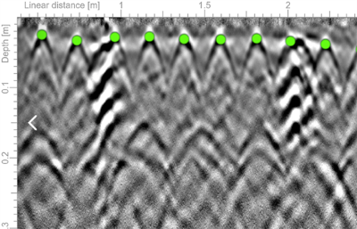
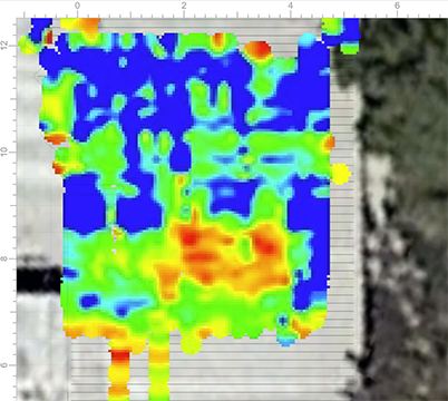
The map of the strength of the hyperbolic reflections for each rebar to map corrosion can be made using the Amplitude grid layer. Care must be taken to ensure that no processing step has normalised the amplitudes of the reflections, such as an AGC gain. In addition, it should be acknowledged that deeper reflections will have lower amplitude and some bias may occur using gain functions to compensate for their lower amplitude. The map below shows low amplitude reflections from rebar (possibly associated with corrosion) in red.
Gridding methods
Geolitix offers the following gridding methods. There is no recommended griding method as each has its uses on a case-by-case basis.
- Kriging is a geostatistical gridding method that has proven useful and popular in many fields. This method produces visually appealing maps from irregularly spaced data. Kriging attempts to express trends suggested in your data, so that, for example, high points might be connected along a ridge rather than isolated by bull's-eye type contours.
- With Inverse Distance Weighted, data are weighted during interpolation such that the influence of one point relative to another decreases with distance from the grid node. Weighting is assigned to data through the use of a power parameter that controls how the weighting factors drop off as distance from a grid node increases. The greater the weighting power, the less effect points far from the grid node have during interpolation
Grid cell size
The grid cell size is the size of each pixel on the resultant slice. As a general guideline, the cell size should not be less than the trace spacing and not be more than half of the spacing between profiles. Very small cell sizes do not improve the resolution of the resultant slices and can slow down processing. Very large cell sizes will result in poor resolution and jagged maps.
Search radius
The search radius refers to the region over which the algorithm looks for data points to create a slice. As a general guideline, it should be on the order of 1.5 times the average line spacing. A small search radius will not “bridge” the gap between adjacent lines and will result in empty pixels, whereas a large search radius will include the effects of data points very distant from the point of interpolation.
Clip borders
Clipping the borders of the resultant slice uses an algorithm to blank all cells outside of the edges of the survey area. This also works if there are multiple survey areas. Without clipping the borders of a slice, the entire bounding box of data will be filled with data, including regions outside of the survey area.
Color schemes
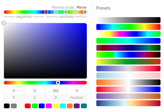
A color scheme can be selected from a series of pre-defined options. You are not limited to the pre-defined options listed. Geolitix allows full control over the color scale using a color picker tool. The tool also enables you to control the minimum and maximum of the color scale.
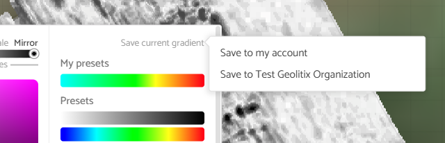
Any color scale can be saved to either the user's account or, in the case of corporate accounts, to the organization's account. This is particularly useful if a specific color scheme is used for a client or as part of corporate branding.
Post-processing of amplitude grids
Use the  to add a post-processing step to the grid.
- Moving average allows you to apply a smoothing filter to the slices to remove high frequency noise. You can select the number of pixels to average over, in both the x and y directions.
- The Histogram Editor displays a histogram of the amplitudes of all the slices in your model. By placing sliders on the histogram, you can increase the brightness of certain ranges of amplitudes or subdue others. This tool is useful in enhancing subtle features to be more visible by essentially increasing the contrast of the slices.
- The Constant scale tool multiplies all slices in a model by a value to increase brightness. A constant scale also increases the brightness of random noise on the slices.