Appearance
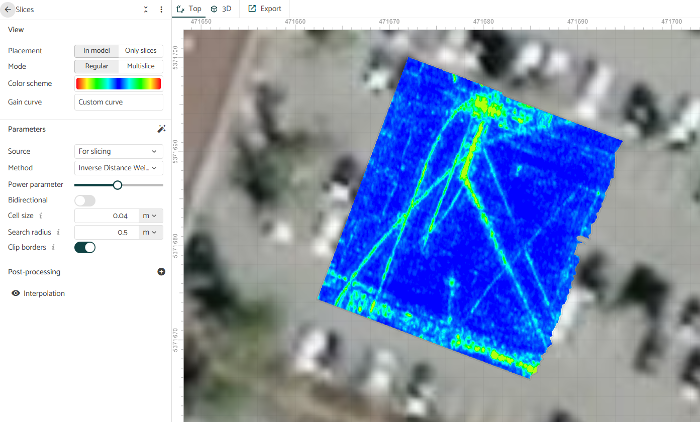
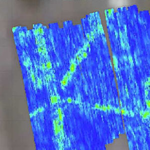
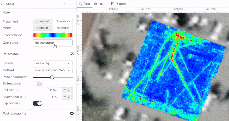
Slices
In GPR terminology, slices refer to horizontal planar slices though a volume of dense GPR data. Slicing works best when there is a close line spacing between GPR profiles, generally on the order of approximately a quarter wavelength. For most GPR applications, this means a grid profile spacing equal to the width of the GPR antenna being used, although for practical reasons, this spacing may be increased.
Adding a Slice layer reveals the slice dialog options.
Slide controls
In the 2D or 3D map view, you can control the slice or multislice depth and thickness with results shown live on the map. A single slice refers to the amplitude of radar reflections at a specific depth (e.g. 1.2 m). The "thickness" of a slice refers the sum of amplitudes between two depth ranges (e.g. from 1.2 m - 1.8 m). The advantage of thick slices is their ability to show dipping pipes or pipes at different depths in one view. However, a thick slice should not be used to determine pipe depth since there is no way of determining where within the depth range the pipe or cable reflection starts.
You can also hold down the SHIFT key and use the mouse scroll wheel to cycle up and down slice depths. This is particularly useful when tracking a dipping pipe or cable.
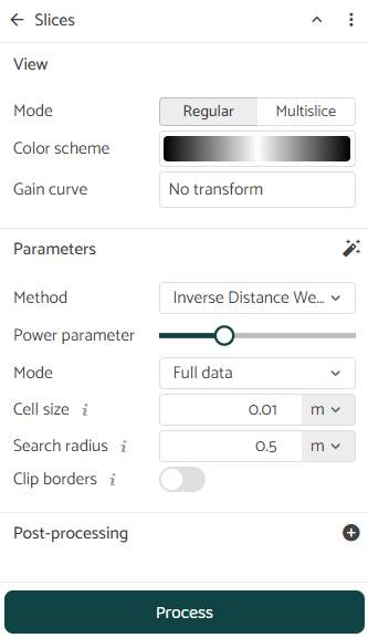
Parameters
Slicing requires you to input a series of parameters to define the gridding method, the cell size (i.e. resolution) and the search radius of the grids for each slice layer. The parameters are functions of the input GPR data and can be calculated by Geolitix automatically1. Clicking the magic wand icon  fills in the gridding parameters with optimal values as calculated by Geolitix.
Source
If there is more than one processing tag applied to the GPR profiles, a drop-down box to select which one is processed for slicing appears. Generally, the processing scheme to be sliced is one which contains migration and the Hilbert transform. When Automated Processing has been applied to the dataset by Geolitix, Slicing should use the processing tag "For slicing".
Method
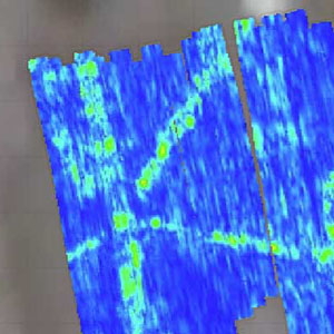
Geolitix offers a number of gridding methods. There is no recommended griding method as each has its uses on a case-by-case basis. Examples as shown of gridding outputs using the same parameters with array GPR data.
Kriging is a geostatistical gridding method that has proven useful and popular in many fields. This method produces visually appealing maps from irregularly spaced data. Kriging attempts to express trends suggested in your data, so that, for example, high points might be connected along a ridge rather than isolated by bull's-eye type contours.
Inverse Distance Weighted data are weighted during interpolation such that the influence of one point relative to another decreases with distance from the grid node. Weighting is assigned to data through the use of a power parameter that controls how the weighting factors drop off as distance from a grid node increases. The greater the weighting power, the less effect points far from the grid node have during interpolation

The Nearest Neighbour gridding method assigns the value of the nearest point to each grid node. This method is useful when data are already evenly spaced but need to be converted to smooth grid. Alternatively, in cases where the data are nearly on a grid with only a few missing values, this method is effective for filling in the holes in the data.
Gridding Mode
The mode selector controls how data points are processed before gridding, with each mode optimized for different survey scenarios and data characteristics.
Full Data uses all available data points in their original form for gridding. This is the standard approach suitable for GPR surveys where the data density is similar in all directions.
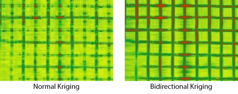
Bidirectional gridding can be useful for scenarios where there are crossing pipes or rebar at right angles. Using bidirectional gridding (sometimes referred to as de-coupled gridding), Geolitix uses an elliptical search radius in the x direction first to create a grid which accentuates pipes or rebar in the x direction. It then creates a grid with accentuation in the y direction. Finally, it adds the two together, resulting in an improved visualization of pipes or rebar at right angles.
- Binning mode creates bins along the profile tracks, averages the data within each bin, and then uses these sparser points for gridding. This approach equalizes the data density both along the profiles and perpendicular to them, resulting in smoother images. Binning is particularly useful when there is a high trace density along profiles but wider spacing between profiles, as it prevents the gridding algorithm from being biased by the denser in-line data.
Grid cell size
The grid cell size is the size of each pixel on the resultant slice. As a general guideline, the cell size should not be less than the trace spacing and not be more than half of the spacing between profiles. Very small cell sizes do not improve the resolution of the resultant slices and can slow down processing. Very large cell sizes will result in poor resolution and jagged maps. For example, if a survey was collected with a trace separation along a profile of 5 cm, then a reasonable grid cell size would be 5 cm.
Search radius
The search radius refers to the region over which the algorithm looks for data points to create a slice. As a general guideline, it should be 1.5 times the average line spacing. A small search radius will not “bridge” the gap between adjacent lines and will result in empty pixels and a large search radius will include the effects of data points very distant from the point of interpolation. 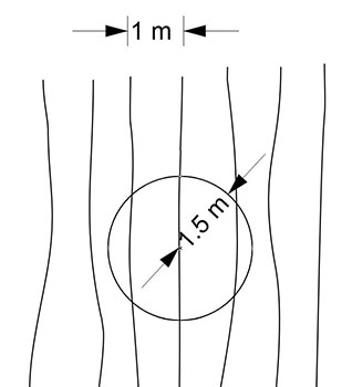
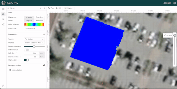
Clip borders
Clipping the borders of the resultant slice uses an algorithm to blank all cells outside of the edges of the survey area. This also works if there are multiple survey areas. Without clipping the borders of a slice, the entire bounding box of data will be filled with data, including regions outside of the survey area.
Visualization Options
Color schemes
A color scheme can be selected from a series of pre=defined options. Since the Hilbert transform filter is generally used for creating data suitable for slicing, it is recommended that the color scheme be mirrored so that it stretches only in the positive scale using the  icon.
icon.
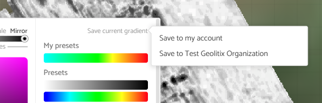
You are not limited to the pre-defined options listed. Geolitix allows full control over the color scale using a color picker tool. The tool also enables you to control the minimum and maximum of the color scale.
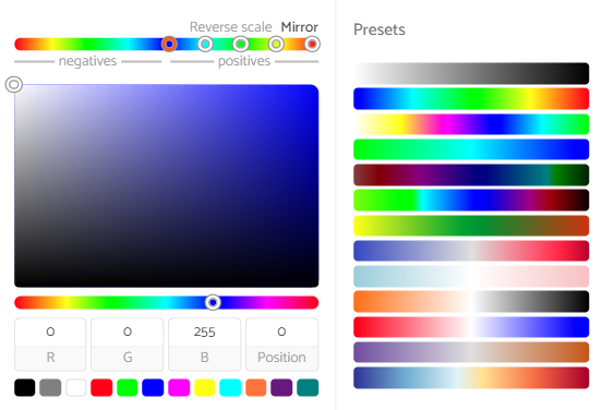
Any color scale can be saved to either the user's account or, in the case of corporate accounts, to the organization's account. This is particularly useful if a specific color scheme is used for a client or as part of corporate branding.
The color scale distribution (gain) is also customisable. Click the Gain curve option to enable to curve editing tool.
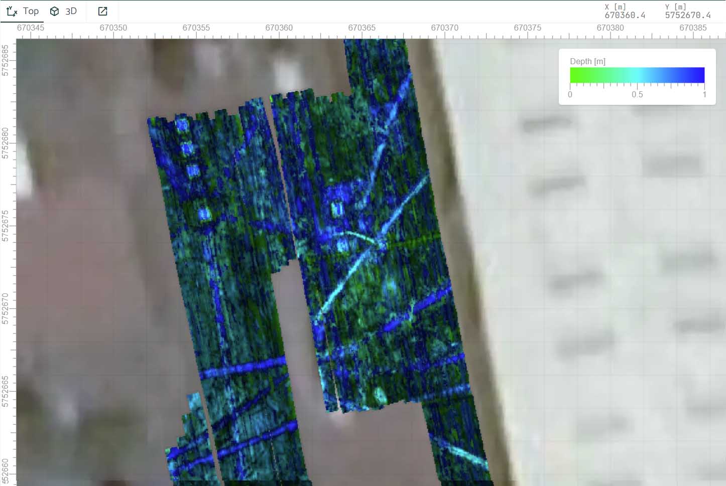
Multislices mode
The multislices mode provides a way to view a range of GPR slices simultaneously using a color scale that represents depth, allowing users to quickly identify features at different levels2. This approach is particularly useful for examining regions with complex linear features such as networks of pipes and cables at various depths. The algorithm analyzes the entire stack of slices and identifies the peak value at each grid location, then represents this peak as a color corresponding to the depth at which it was found. While direct interpretations should normally not be made from multislice displays, this visualization serves as an effective final check to ensure that all features within the dataset have been properly identified and accounted for.
Post-processing of slices
Use the  to add a post-processing step to slices.
- Interpolate slices uses bilinear interpolation to calculate colors on the slices. Bilinear interpolation makes the color gradations smoother.
- Normalize slices stretches the dynamic range of each slice to the full extent of the color spectrum. For example, if your data has a few layers of very amplitude reflections which so brightly on slices and other layers where there is no data visible, normalizing slices will make all layers equally bright. This will enable the mapping of weaker targets when strong targets are present, but you can no longer discern “strong” from “weak”, since all reflections will be strong.
- Moving average allows you to apply a smoothing filter to the slices to remove high frequency noise. You can select the number of pixels to average over, in both the x and y directions.
- The Histogram Editor displays a histogram of the amplitudes of all the slices in your model. By placing sliders on the histogram, you can increase the brightness of certain ranges of amplitudes or subdue others. This tool is useful in enhancing subtle features to be more visible by essentially increasing the contrast of the slices.
- The Constant scale tool multiplies all slices in a model by a value to increase brightness. A constant scale also increases the brightness of random noise on the slices.
References
- Luo et al. (2019) GPR Imaging Criteria, Journal of Applied Geophysics (165) 37-48
- Grasmueck, M. and Viggiano, D. (2018) PondView: Intuitive and Efficient Visualization of 3D GPR Data, IEEE International Conference on Ground Penetrating Radar (GPR), pp. 1-6