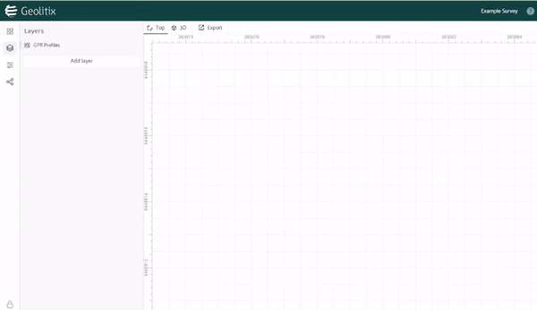
Appearance
GPR Processing
All GPR data requires some form of processing or filtering to enhance detectability of the desired targets. It is not the purpose of this document to detail all possible processing scenarios and steps, as these are learned by experience within the context of the survey environment, purpose and equipment. Each GPR survey will have its own personal preferences on data presentation.
Some GPR systems (e.g. some older GSSI systems) apply processing filters directly to the data as it is collected. In these cases, it is important that the GPR surveyor be aware of the processing and filtering being applied and that it cannot easily be undone. The use of the wrong filter may result in useless data.
Automatic GPR Processing
Geolitix has the ability to analyze input GPR data and devise a processing scheme to maximise interpretability. Automated processing is available at any time during workflow but is best enacted during import of raw data. Upon import of any GPR data, Geolitix will present you with an option to manually proceed or begin automatic processing.
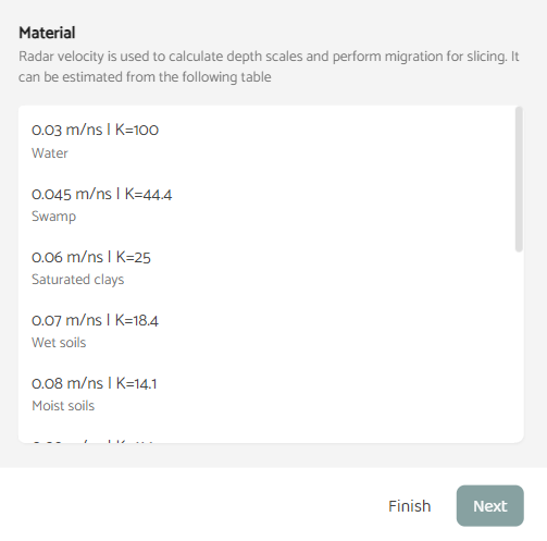
Clicking Finish at this dialog will allow you to manually process the GPR data, whereas Next will continue allowing Geolitix to automatically process and present the data, along with automated slices if applicable. Although most steps of GPR processing can be automated by analyzing the data, the radar velocity must be set by you. The next screen in the dialog asks you to select a suitable velocity and provides some sample soil types for each option. If unknown, a velocity of 0.1 m/ns represents typical moist soils.
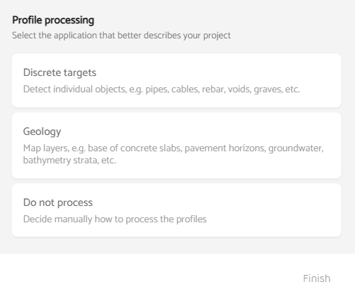
Geolitix then asks you to define the objectives of the survey. If the mapping of pipes, cables, rebar or other discrete objects is the primary objective, then slicing will be automatically performed if you wish. Slices will be made for each antenna frequency or antenna orientation for multichannel radars. If the objective is to map layers of geology or pavement, then no slicing is performed. You may also opt to not automatically process the GPR data.
Once processed, Geolitix displays all slices and processed GPR profiles. The GPR profiles will show two types of processing in the processing tabs: one for regular processing and one for slicing, which includes migration and a Hilbert transform.
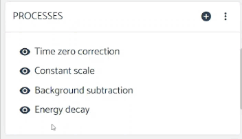
Processing steps
Individual processing steps can be added by pressing the plus icon  and deleted with the garbage can icon
  .
.
Processing steps are global (they apply to all files in a project automatically), unless the globe icon is pressed  . In this case, the process will only be applied to the profile shown and that processing step will have a warning stating that the step was applied only to that profile.
Almost all processing steps can be re-ordered at any time. The exceptions are set time zero, remove idle traces, remove empty traces, mute traces, trace shifting, and resample traces equidistantly, which must always be at the top of the processing list. This is because they affect positioning and thus must be performed first.
Processing groups
Geolitix defines a list of processing steps as a processing group. Sometimes, you may wish to experiment with different processing steps or order of steps. This can easily be done by either creating a new processing group from scratch or duplicating an existing processing group, by selecting the options icon  . You may have as many processing groups as you’d like, and these can be renamed as required. This is particularly useful when slicing and showing profiles with hyperbolas at the same time.
GPR processing in Geolitix is divided into those which manipulate data in the time domain (along the time axis), in the spatial domain (along the x axis), as well as filters which operate in either or both domains.
TIP
Data appears all grey? Many manufacturers save data in 32 bits, but do not use the full range of 32 bits. Thus all of the data are relatively low amplitudes compared to the full 32 bit scale, and are displayed as grey on a greyscale. To see your data, add a constant scale or normalisation processing step.
Processing as function of time
Trace shifting
Some radars can record data with first arrival shifts. This was common in older GPR units which needed to be warmed up before the timing circuits became stable. To correct for time zero jitter or drifts, use the Trace shifting step and adjust the slider until the first arrival is flat. 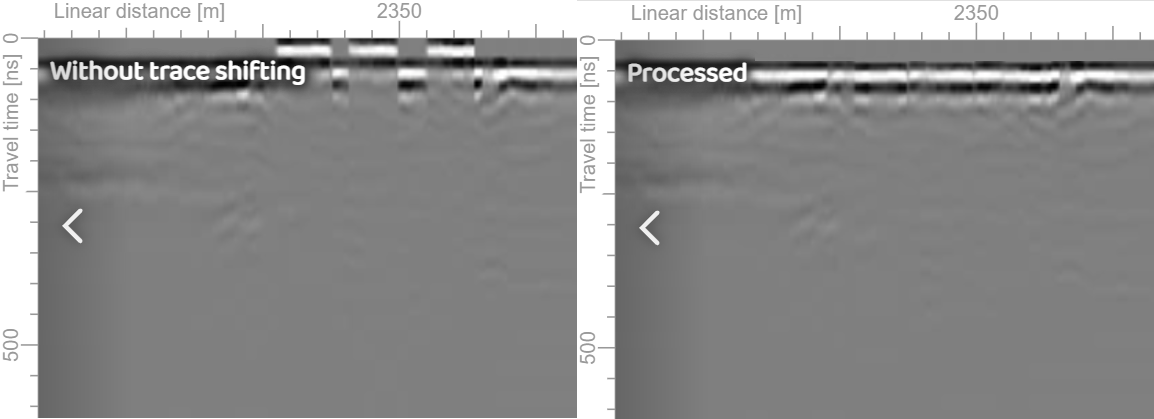
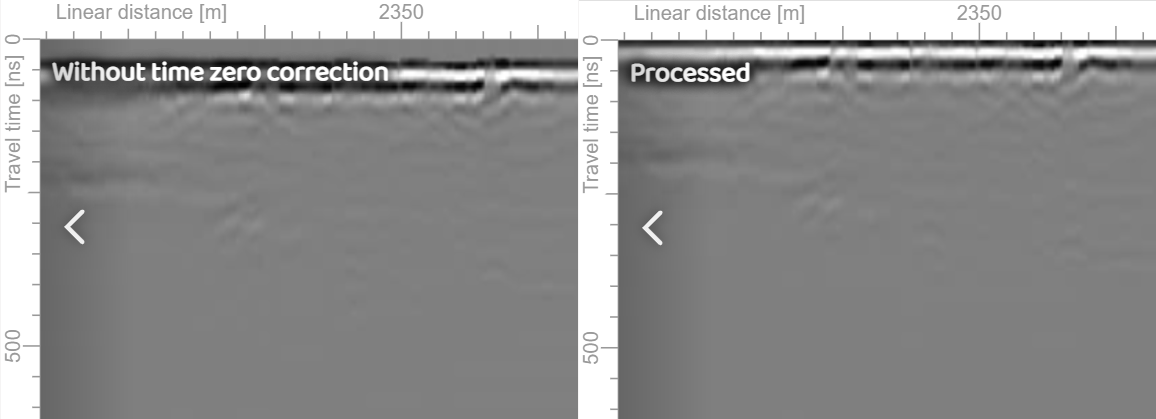
Time zero correction
Data from all GPR systems must have the portion of the profile above time zero removed. Most radar systems display data without time zero on the field software, but this “dead” time must be removed in post processing. Before time zero, the signal is internal to the radar system and not related to the ground reflections. If time zero was not removed, all depth information would be incorrect.
| Parameter | Details |
|---|---|
| Method | Set threshold. Finds first sample over the selected threshold. Find peak. Finds sample with higher amplitude. Set travel time. Manually select the travel time. |
| Backup samples | Selectable number of samples to fine tune the time zero setting |
| Trace by trace | If selected, the correction is applied on a trace by trace basis instead of shifting the entire profile by the same amount |
Resample
This allows you to resample data traces in the time domain, usually to interpolate a finer time increment. This process should be applied sparingly and in no way improves the resolution of the radar. On some deep radar systems with coarse time sampling, resampling the data may improve interpretability.
Time cut
This step allows you to trim the radar profile, either from the top or from the bottom, using the pull-down menu. The slider allows you to set the number of ns of the final time window. This step is often useful if the time range was set too large during data collection (i.e too deep) and you wish to focus processing on a specific depth only.
Flatten to horizon
In some situations (e.g. drone GPR, other air launched antennas and surveys done on thick snow), variations of the antenna height above the ground need to be accounted for. This is not a simple time zero correction along a first break. You can manually draw in the ground surface reflection or use the automated horizon picking tool and then use this process to correct your data to be flat to the ground surface. 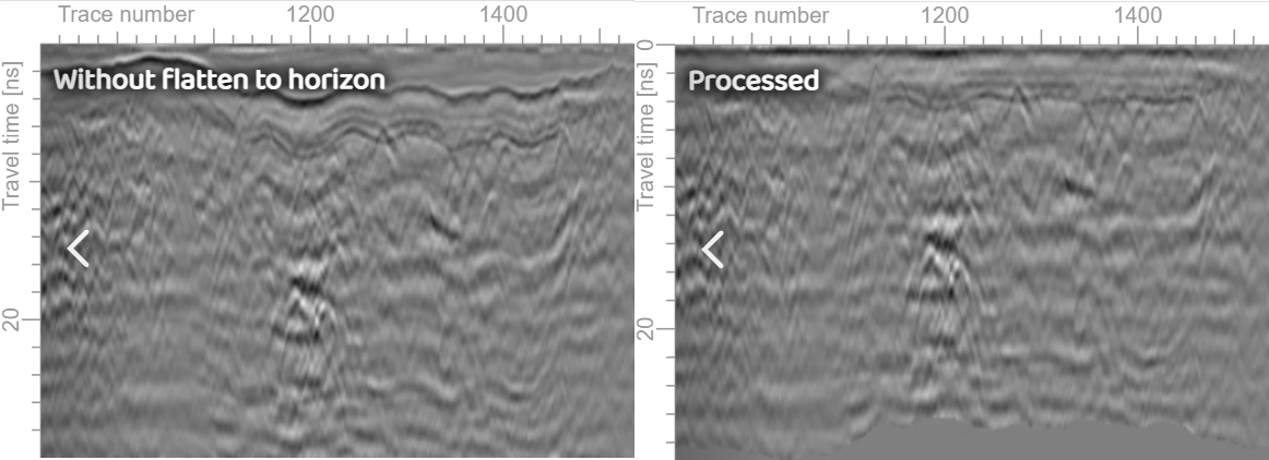
Processing as a function of traces (distance)
Remove idle traces
When collecting data using GPS and without triggering from an odometer, the radar is often stationary but continues collecting data. These “idle” traces can be deleted using this step. The user sets a threshold value to search for such traces. 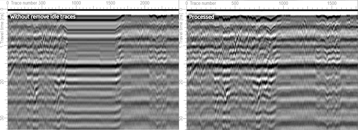
Remove empty traces
Errors on some GPR systems can cause traces with no data to be recorded. With this processing step, Geolitix searches for traces with no data and removes them from the profile automatically. 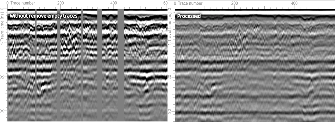
Remove traces
To remove unwanted segments of a profile, the remove traces step can be used. Use the pencil  and garbage can
  icons to highlight the traces to be removed.
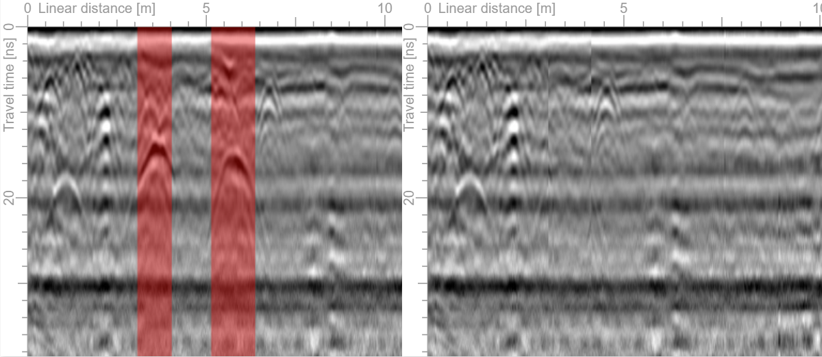
Mute traces
In some situations, you may wish to mute, or hide, some traces, but maintain the correct length of the profile. This may occur when the radar has passed over a metal plate, creating a distracting strong ringing effect to the bottom of the trace. In other situations, you may wish to mute out traces with excessive interference. This can be done in Geolitix using the Mute trace step. Use the pencil and garbage can icons to highlight the traces to be removed. 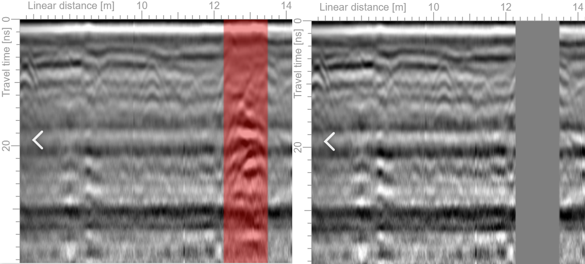
Resample traces equidistantly
Data collected with GPS tracking might require spatial resampling if we wish all traces to have the same width. This is because data were collected at different speeds. Even if there was an odometer used to trigger the radar, the data still needs to be “rubbersheeted” to match the desired trace spacing increment.
Resampling traces equidistantly allows you to specify a trace separation using an interpolation algorithm. If the separation is less than the distance between traces as measured by the GPS, then new traces will be added to ensure a constant trace separation is maintained. Conversely, traces will be lost if the desired separation is greater than the distances measured by the GPS. 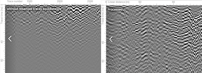
Gain functions
As radar signals penetrate the ground a portion of the energy is attenuated, and a portion is reflected back to the surface. Therefore, with increasing depth, the signal strength diminishes. A gain function is applied to each trace to compensate for this attenuation. There is no single gain function which works best for every scenario.
The goal of gaining your radar profile is to make all the targets as visible as possible amongst the noise inherent in the data.
Constant scale
This is the simplest type of gain, whereby a multiplier is applied equally down each trace. This gain is useful when viewing data from some manufacturers who do not use the full resolution for their data. In these cases, the radar profile appears entirely grey until a constant scale gain is applied. You can control the amount of constant gain with the sliding scale. 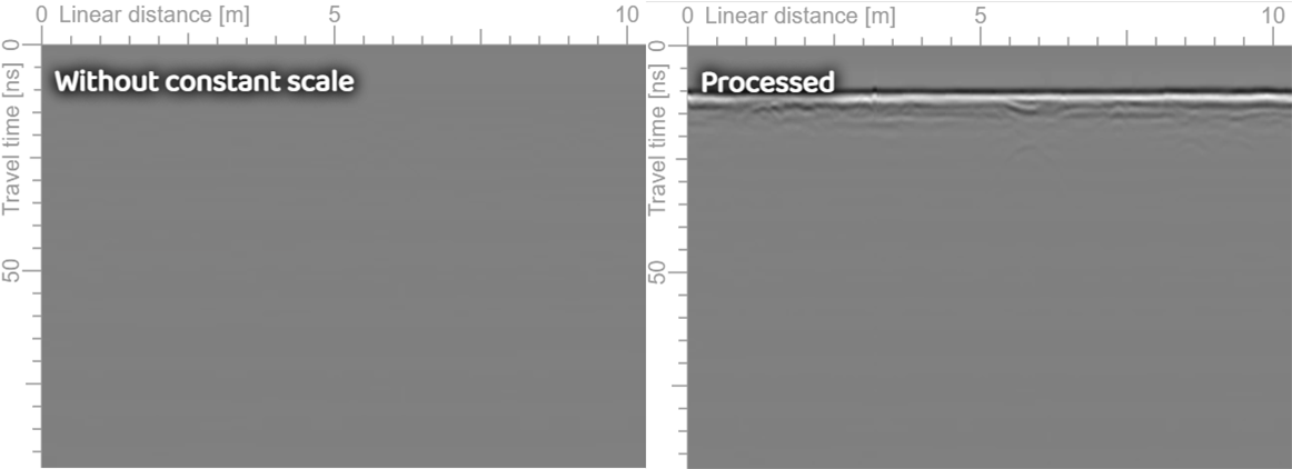
Normalization
A normalization gain can be applied on a trace-by-trace basis, or to an enter profile. During normalization, each trace or profile is scaled to its maximum value. In the case of raw data which are of low amplitude, effectively trims the unused edges of the data scale, allowing you to see the data. However, if there is a few traces of very high amplitude (e.g. if the radar passed over a metal plate), then the normalization function will be scaled to those high amplitudes and the remainder of the profile will still not be visible. Such outlier traces can be ignored. 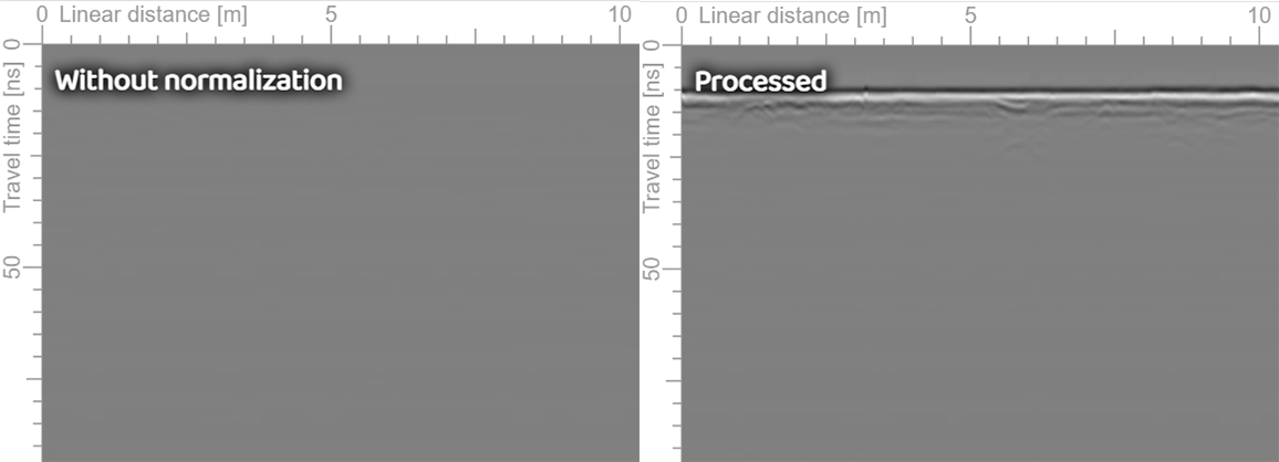
Automatic gain control (AGC)
This gain attempts to create an equal distribution of amplitudes in the time domain within a user-definable window. It must be noted that all relative amplitude information is lost using AGC, and we can no longer state that a certain target has a “strong” or “weak” reflection.
The sample window determines is set by you. The average amplitude is calculated over the entire trace, and each sample amplitude is then scaled so that the mean amplitude has the same value for each selected sample window around the current value within a trace. Small window sizes cause strong equality distributions, whereas large windows cause weaker distributions. 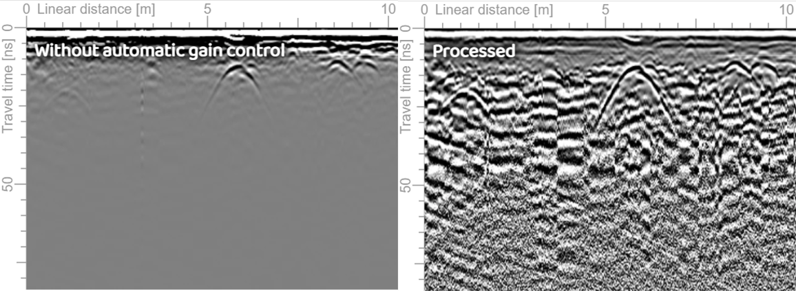
Energy decay gain
An energy decay gain involves applying a gain to the complete profile based on the mean amplitude decay curve. The algorithm first calculates the mean decay curve for all traces in a profile and then applies a gain to each trace to compensate for the mean decay. This type of gain is generally the most useful in most situations, but care must be taken if your profile(s) have very high reflection values such as passing the radar antennas over a metal plate. This can change the mean curve, causing the rest of the profile to be weak in amplitude. In addition, the energy decay gain operates on a profile-by-profile basis. A profile with a particularly strong reflection (e.g a manhole cover) can cause strong striping in slices. A solution for this is to convert the Energy decay gain into a manual gain using the button on the energy decay settings. 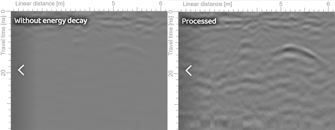
Manual gain
Rather than a calculated gain, you may wish to draw a gain curve yourself, enabling you to highlight specific depths or layers. Click on the graph to draw points for the desired curve, with the effects shown on the profile window. You can subdue time regions with a negative dB gain or enhance regions. To gain beyond the scale shown, press the plus icon on the graph. An example manual gain curve may look like this.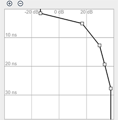

Linear gain
A linear gain simply applies a time-varying gain which increases linearly with depth. You can control the amount of linear gain with the sliding scale. 
Exponential gain
An exponential gain applies increasing amounts of gain with increasing depth. Since radar attenuation is generally exponential with depth, compensating by an exponential function makes sense. You can control the start time of the gain as well as the degree of exponential gain. 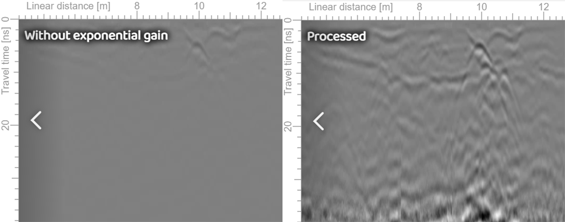
Attenuate by horizon
In some scenarios, you may with to draw attention to a specific layer or subdue reflections above or below a geological horizon. An example of this may be bathymetry surveys where noise and reflections within the water column may be distracting to the viewer. This can be achieved by using the interpretation tool to draw a continuous horizon across a profile, and then applying this process to subdue data above or below that interpreted line. You can adjust the amount of edge fade on this effect. 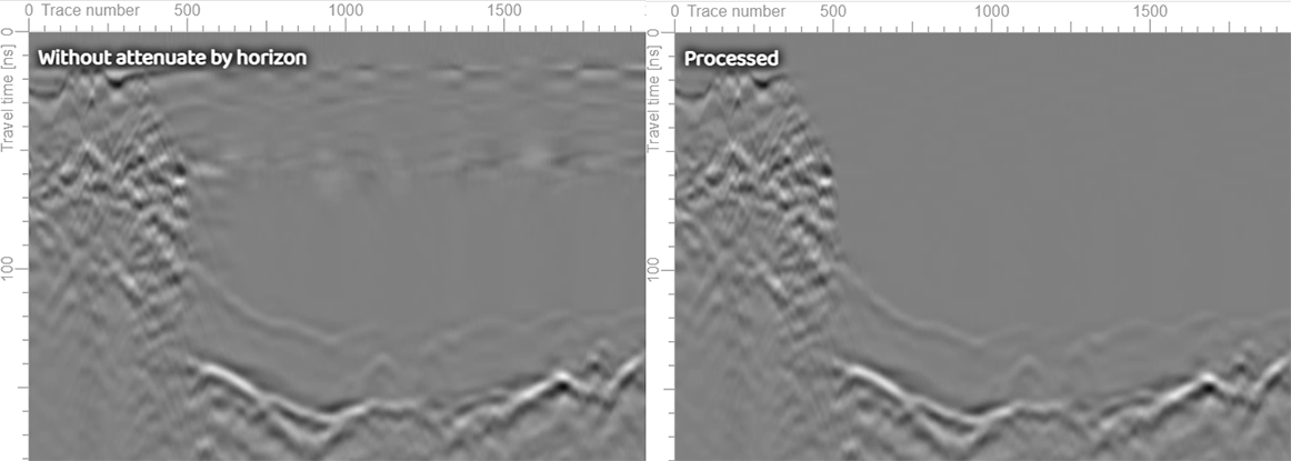
Gamma correction
A gamma correction adjusts the contrast of a profile. It is not a gain as such but can be used to highlight strong reflectors. 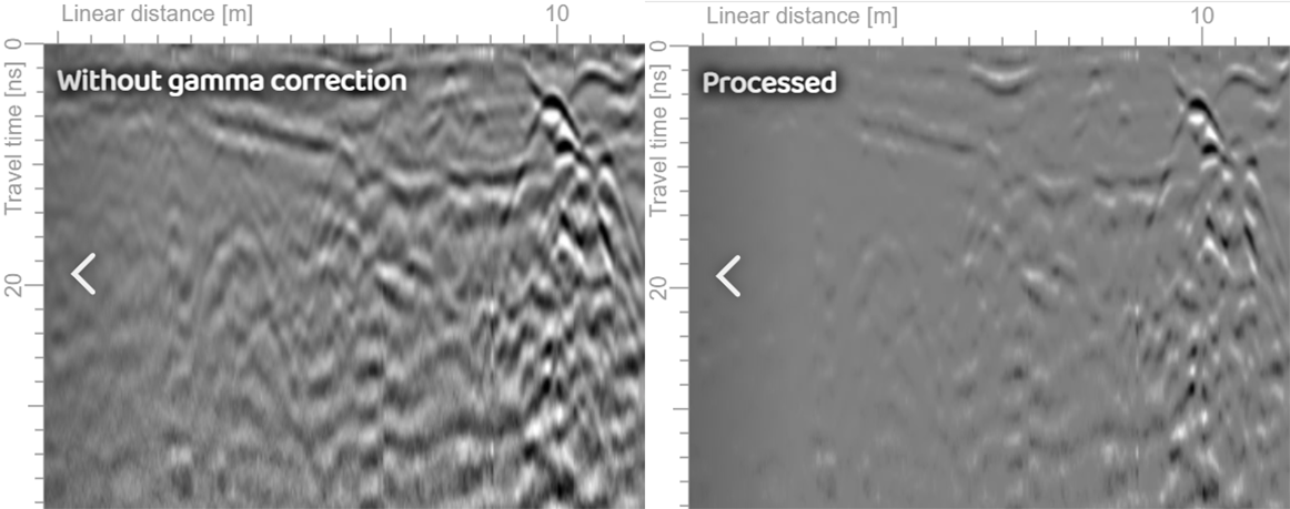
Filters
Frequency filter
These filters act in one dimension, meaning that they act on a trace-by-trace basis. They are useful in reducing noise in a GPR profile. Most GPR antennas have a bandwidth of approximately the same as their center frequency. That is, a 500 MHz antenna would have an effective bandwidth from 250 MHz – 750 MHz. Data recorded below about 250 MHz is often a function of background noise, and data recorded above 750 MHz is often due to instrument noise. A high-pass filter will eliminate data below a cut-off value, and a low-pass filter will eliminate data above a cut-off value. An alternative approach is to use a band pass filter, in this case between 250 MHz – 750 MHz. Conversely, a band stop filter will eliminate data between a lower and higher frequency.
The filter order effects the sharpness of the cut-off of the filter.
A notch filter is similar to a band stop filter in that it attenuates frequencies within a specific range while passing all other frequencies through. However, a notch filter is much narrower and deeper. It is most useful for eliminating interference at a specific frequency caused by a mobile phone or similar radio. 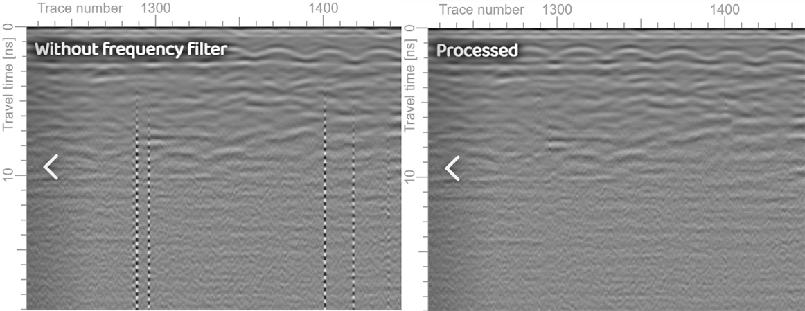
2D FFT
2D FFT filtering is most commonly used in image processing but can be very powerful when filtering noisy GPR data where there are repeating patterns such as air-wave reflections all dipping at the same angle. Even antenna ringing, which is a repetitive pattern, can be effectively removed using 2D FFT filters.
In this example, the filter shown below is used to subdue the dipping reflectors on the radar profile caused by above-ground reflections. 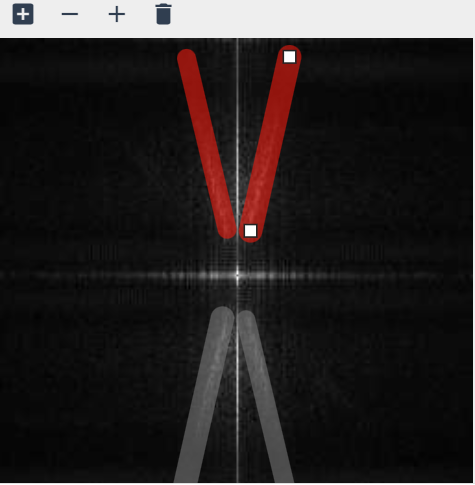
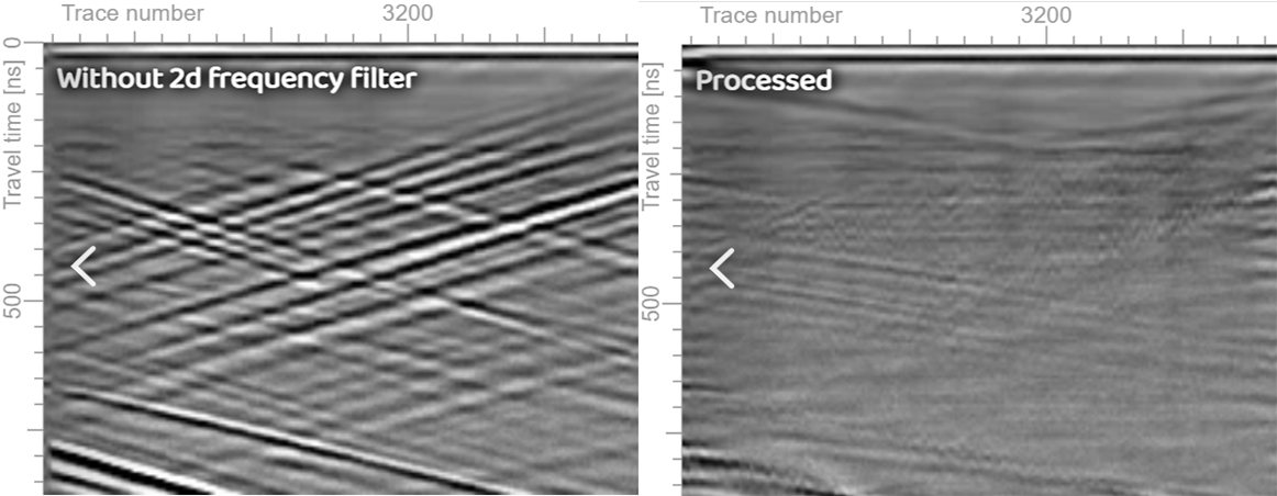
To create the FFT mask, use the  icon. To thicken or thin the masking line, use the + and – buttons.
Background subtraction
Background removal is used to enhance the visibility of the desired radar targets but eliminating horizontal lines in the data. These lines are often caused by ringing in the antennas or within the antenna shields. The most common method of background removal is to subtract from each trace an average of a trace window on either side of it. The user is able to select the size of the window. 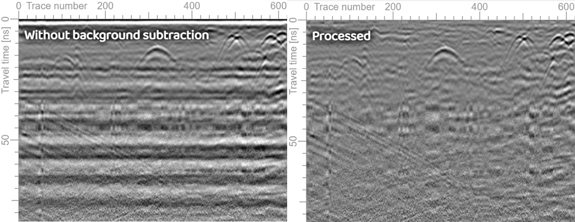
However, a special issue arises when there is a very strong vertical reflection, such as when the radar antenna was passed over a metal plate. If an average subtraction is used, then the strong reflections will be blurred on either side of the plate, distorting the data. Geolitix offers a remove median function for such situations. The comparative effects of these two variations of filters are shown below. 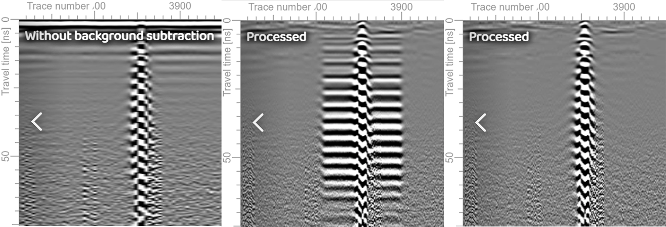
Dewow
When most GPR systems record raw data, there is a component of the data known as “wow”. These are inductive effects from the antenna coupling with the ground, or instrumentation dynamic range limitations, and manifest themselves as a very low frequency component of the radar profile. These effects can be removed using a dewow filter. The dewow effect is calculated over a user-defined window. Too small a value essentially is a high pass filter whereby only the high frequency components of the profile remain, and too large a value results in no change to the profile. The user can employ the slider to select the optimal degree of dewow. 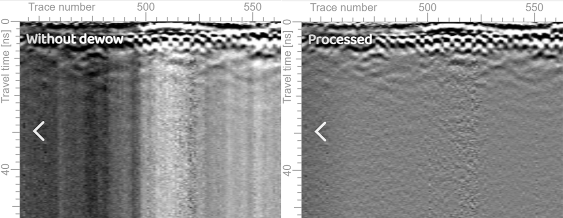
Moving average
A moving average filter applies a vertical (down-the-trace) and/or horizontal (trace-to-trace) smoothing operation to a GPR profile. The amplitude at any point on the profile is replaced by the data value at a given point by the averaging window. This is commonly employed to reduce random high frequency noise and acts similar to a low-pass filter. 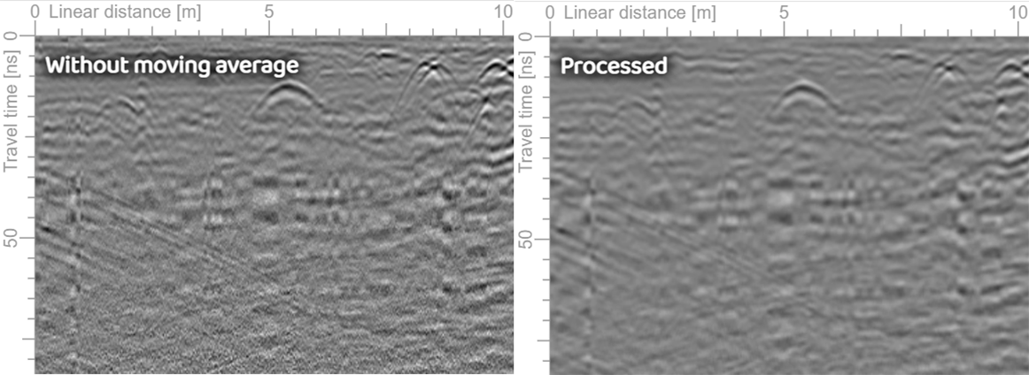
Gaussian blur
Blurring is commonly used for smoothing effects when digitally editing photos and videos. Unlike an averaging filter, a Gaussian smoothing filter weights the center of the filter greater than the outer edges. 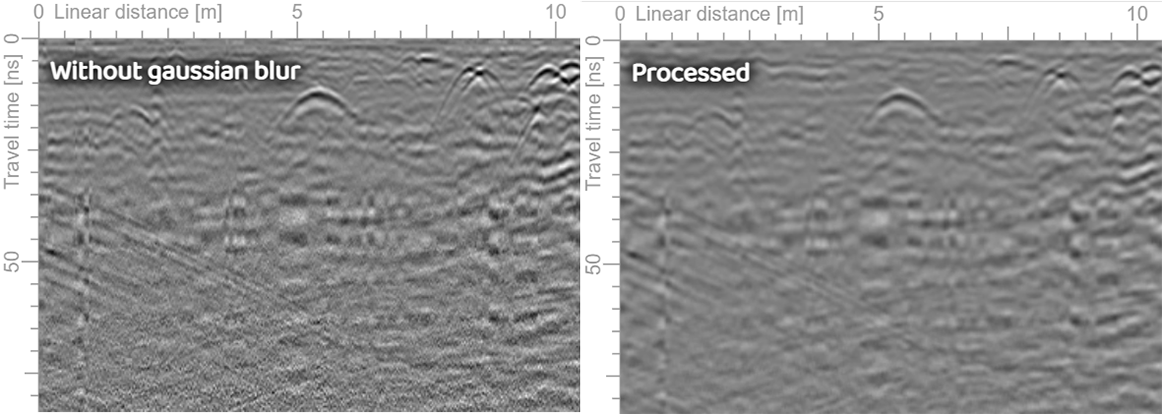
Sobel transform
The Sobel operator is used in image processing as an edge detector. It computes an approximation of the gradient of the image intensity function. It is most useful in mapping stratigraphic layers on GPR profiles, such as sedimentary horizons or the thickness of ice and snow. 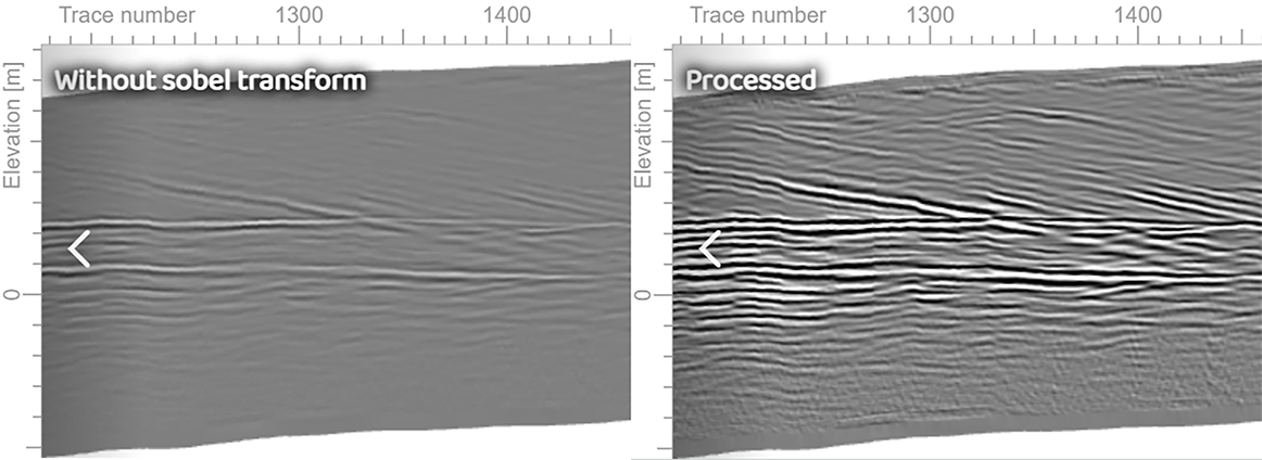
Texture analysis
This function performs a textural analysis of radar profiles to highlight regions of similar reflection shapes and directions. It is most useful in geological mapping applications where complex layers can be discerned more easily by studying variations in texture rather than layer reflections. 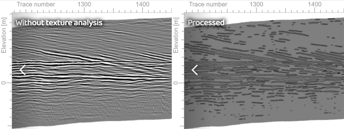
Hilbert transform
The Hilbert transform replaces each trace with its envelope, effectively removing its negative component. This step is commonly used after migration when creating slices of GPR datasets to highlight discrete targets. 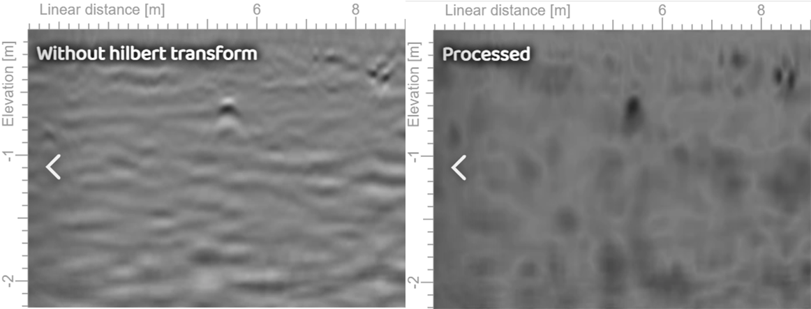
Migration
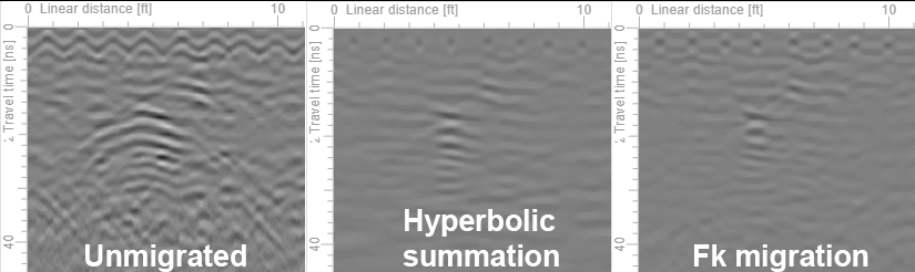
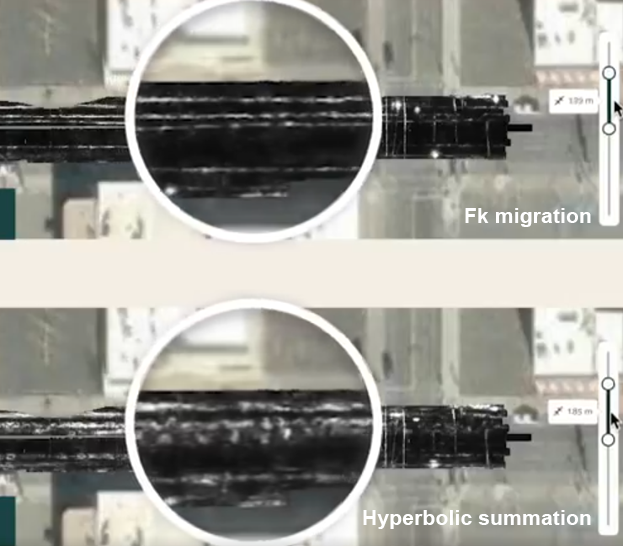
Migration is used to collapse the energy contained in a hyperbolic reflection of a discrete object into a single point. The user must first have entered in the project velocity or have calculated the velocity using the adaptive hyperbola tool.
Geolitix provides two types of migration. The hyperbolic summation method sums along the hyperbolic shapes to focus the energy back to the apex of the hyperbola. The FK migration method aims to move dipping reflectors to their true subsurface positions and collapse hyperbolic diffractions to points, working by applying a phase shift in the frequency-wavenumber domain based on the wave equation. Each of these methods have benefits and limiations. In general, 3D FK migration should be used with all array datasets, and more sparse single channel data can use either 2D method. Note that the presence of metal objects (e.g. manhole covers) can create large artifacts in FK-migrated data. It is recommended that a Remove metal reflections function be used prior to FK migration.
Absolute value
This function replaces the amplitude of each sample with its absolute value.
Subtract DC shift
This function subtracts a time-constant shift to each separate trace. The average value is calculated between your selected range and subtracted from all samples of each trace.
Remove outlier samples
This function removes traces with excessive noise due to instrument errors or high interference. The user selects the threshold of deviation from the mean trace to remove.
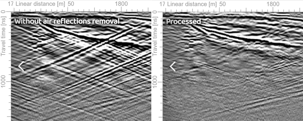
Remove air-wave reflections
Both shielded and unshielded antennas can suffer from above-ground reflections. These are caused by the emitted radio waves reflecting off trees, buildings, people, cars etc. This process can be used to attenuate such reflections. It is moset effective at removing distant air-wave reflections.